Part 3: NNMM with Intermediate Omics Features

Model Architecture

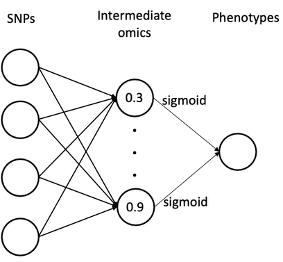
When you have observed intermediate omics data (e.g., gene expression, metabolomics), NNMM can incorporate them in the middle layer:

Genotypes → (Complete/Incomplete) Intermediate Omics → Phenotypes
 (Layer 1)              (Layer 2)                       (Layer 3)

Example: Fully-Connected Network with Observed Omics

This example demonstrates:

• Activation function: sigmoid (other options: "tanh", "relu", "leakyrelu", "linear")
• Number of omics features: 10
• Bayesian model: BayesC for marker effects
• Missing omics handling: Hamiltonian Monte Carlo

# Step 1: Load packages
using NNMM
using NNMM.Datasets
using DataFrames
using CSV
using Statistics
using Random

Random.seed!(123)

# Step 2: Load simulated dataset
geno_path = Datasets.dataset("genotypes_1000snps.txt", dataset_name="simulated_omics_data")
pheno_path = Datasets.dataset("phenotypes_sim.txt", dataset_name="simulated_omics_data")

# Read data
pheno_df = CSV.read(pheno_path, DataFrame)

# Step 3: Prepare omics file (Layer 2)
# Select ID and 10 omics features
omics_cols = vcat(:ID, [Symbol("omic$i") for i in 1:10])
omics_df = pheno_df[:, omics_cols]
omics_names = names(omics_df)[2:end]  # ["omic1", "omic2", ..., "omic10"]

omics_file = "omics_data.csv"
CSV.write(omics_file, omics_df; missingstring="NA")

# Step 4: Prepare phenotype file (Layer 3)
trait_df = pheno_df[:, [:ID, :trait1]]
trait_file = "phenotypes_data.csv"
CSV.write(trait_file, trait_df; missingstring="NA")

# Step 5: Define layers
layers = [
    # Layer 1: Genotypes
    Layer(
        layer_name = "genotypes",
        data_path = [geno_path]
    ),
    # Layer 2: Omics (with observed values)
    Layer(
        layer_name = "omics",
        data_path = omics_file,
        missing_value = "NA"
    ),
    # Layer 3: Phenotypes
    Layer(
        layer_name = "phenotypes",
        data_path = trait_file,
        missing_value = "NA"
    )
]

# Step 6: Define equations
equations = [
    # Genotypes → Omics (BayesC)
    Equation(
        from_layer_name = "genotypes",
        to_layer_name = "omics",
        equation = "omics = intercept + genotypes",
        omics_name = omics_names,  # Names of omics columns
        method = "BayesC",
        estimatePi = true
    ),
    # Omics → Phenotypes (sigmoid activation)
    Equation(
        from_layer_name = "omics",
        to_layer_name = "phenotypes",
        equation = "phenotypes = intercept + omics",
        phenotype_name = ["trait1"],
        method = "BayesC",
        activation_function = "sigmoid"
    )
]

# Step 7: Run analysis
out = runNNMM(layers, equations;
    chain_length = 5000,
    burnin = 1000,
    printout_frequency = 2000,  # Print every 2000 iterations
    output_folder = "nnmm_omics_results"
)

# Step 8: Check accuracy
ebv = out["EBV_NonLinear"]

# Convert ID types for joining (EBV IDs may be of type Any)
ebv.ID = string.(ebv.ID)
pheno_df.ID = string.(pheno_df.ID)

# If true breeding values available:
if hasproperty(pheno_df, :genetic_total)
    results = innerjoin(ebv, pheno_df[:, [:ID, :genetic_total]], on=:ID)
    accuracy = cor(Float64.(results.EBV), results.genetic_total)
    println("Prediction accuracy: ", round(accuracy, digits=4))
end

# Cleanup
rm(omics_file, force=true)
rm(trait_file, force=true)

Including Residual Polygenic Effects

To include a residual polygenic component (genetic effects not mediated by omics), add an extra latent node to the middle layer:

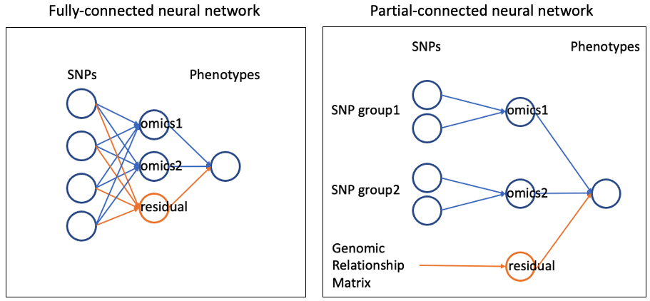
Example: Network with Residual Polygenic Effect

# Step 1: Load packages
using NNMM
using NNMM.Datasets
using DataFrames
using CSV
using Statistics
using Random

Random.seed!(123)

# Step 2: Load data
geno_path = Datasets.dataset("genotypes_1000snps.txt", dataset_name="simulated_omics_data")
pheno_path = Datasets.dataset("phenotypes_sim.txt", dataset_name="simulated_omics_data")
pheno_df = CSV.read(pheno_path, DataFrame)

# Step 3: Create omics file WITH an extra "residual" column (all missing)
omics_cols = vcat(:ID, [Symbol("omic$i") for i in 1:10])
omics_df = pheno_df[:, omics_cols]

# Add residual column (all missing - will be sampled)
omics_df[!, :residual] = fill(missing, nrow(omics_df))

omics_names = names(omics_df)[2:end]  # ["omic1", ..., "omic10", "residual"]

omics_file = "omics_with_residual.csv"
CSV.write(omics_file, omics_df; missingstring="NA")

# Step 4: Create phenotype file
trait_df = pheno_df[:, [:ID, :trait1]]
trait_file = "phenotypes_data.csv"
CSV.write(trait_file, trait_df; missingstring="NA")

# Step 5: Define layers
layers = [
    Layer(layer_name = "genotypes", data_path = [geno_path]),
    Layer(layer_name = "omics", data_path = omics_file, missing_value = "NA"),
    Layer(layer_name = "phenotypes", data_path = trait_file, missing_value = "NA")
]

# Step 6: Define equations (11 features: 10 omics + 1 residual)
equations = [
    Equation(
        from_layer_name = "genotypes",
        to_layer_name = "omics",
        equation = "omics = intercept + genotypes",
        omics_name = omics_names,  # Includes "residual"
        method = "BayesC",
        estimatePi = true
    ),
    Equation(
        from_layer_name = "omics",
        to_layer_name = "phenotypes",
        equation = "phenotypes = intercept + omics",
        phenotype_name = ["trait1"],
        method = "BayesC",
        activation_function = "sigmoid"
    )
]

# Step 7: Run analysis
out = runNNMM(layers, equations;
    chain_length = 5000,
    burnin = 1000,
    output_folder = "nnmm_residual_results"
)

# Step 8: Check accuracy
ebv = out["EBV_NonLinear"]

# Convert ID types for joining
ebv.ID = string.(ebv.ID)
pheno_df.ID = string.(pheno_df.ID)

if hasproperty(pheno_df, :genetic_total)
    results = innerjoin(ebv, pheno_df[:, [:ID, :genetic_total]], on=:ID)
    accuracy = cor(Float64.(results.EBV), results.genetic_total)
    println("Prediction accuracy: ", round(accuracy, digits=4))
end

# Cleanup
rm(omics_file, force=true)
rm(trait_file, force=true)

Handling Missing Omics Data

NNMM automatically handles missing omics values in the training set. Missing values are sampled using HMC based on:

1. The upstream genotype layer (marker effects)
2. The downstream phenotype layer (via backpropagation)

Setting Missing Values Manually

# Convert column type to allow missing values
omics_df[!, :omic1] = convert(Vector{Union{Missing, Float64}}, omics_df[!, :omic1])

# Set specific values to missing
omics_df[10:15, :omic1] .= missing  # Set rows 10-15 as missing for omic1

# Set phenotypes for testing individuals as missing
pheno_df[!, :trait1] = convert(Vector{Union{Missing, Float64}}, pheno_df[!, :trait1])
pheno_df[90:100, :trait1] .= missing  # Testing individuals

Output Files

The output files are the same as described in Part 2, with omics names replacing latent node names.

Tips

1. Many omics features: For large numbers of omics (>100), set printout_frequency to a large value to reduce console output.

2. Pre-processing: Center and scale omics data before running NNMM for better convergence.

3. Testing individuals: Include individuals without phenotypes if they have omics data - this improves the genotype→omics model.

4. Residual effects: Add a completely missing "residual" column to capture genetic variance not explained by omics.