Part 1: Introduction to NNMM
This documentation reflects NNMM.jl v0.3+ using the Layer/Equation/runNNMM API.
1. Overview
The Mixed Effect Neural Networks (NN-MM) extend linear mixed models ("MM") to multilayer neural networks ("NN") by adding one middle layer between the genotype layer and phenotypes layer. Nodes in the middle layer represent intermediate traits, e.g., the known intermediate omics features such as gene expression levels can be incorporated in the middle layer. These three sequential layers form a unified network.

NN-MM allows any patterns of missing data in the middle layer, and missing data will be sampled. In the figure above, for an individual, the gene expression levels of the first two genes are 0.9 and 0.1, respectively, and the gene expression level of the last gene is missing to be sampled. The missing patterns of gene expression levels can be different for different individuals.
2. Extend Linear Mixed Model to Multilayer Neural Networks
Multiple independent single-trait mixed models are used to model the relationships between the input layer (genotypes) and middle layer (intermediate traits). Activation functions in the neural network are used to approximate the linear/nonlinear relationships between the middle layer (intermediate traits) and output layer (phenotypes). Missing values in the middle layer (intermediate traits) are sampled by Hamiltonian Monte Carlo based on the upstream genotype layer and downstream phenotype layer.
Architecture Summary
┌─────────────┐     ┌─────────────┐     ┌─────────────┐
│  Genotypes  │ ──► │   Omics     │ ──► │ Phenotypes  │
│  (Layer 1)  │     │  (Layer 2)  │     │  (Layer 3)  │
└─────────────┘     └─────────────┘     └─────────────┘
     SNPs           Gene Expression        Traits
                    Metabolomics
                    (can be missing)
Key Components
| Component | Description |
|---|---|
| Layer 1→2 | Bayesian regression (BayesA, BayesB, BayesC, etc.) |
| Layer 2→3 | Activation function (linear, sigmoid, tanh, etc.) |
| Missing omics | Sampled via Hamiltonian Monte Carlo |
Details can be found in our publications:
- Tianjing Zhao, Jian Zeng, and Hao Cheng. Extend mixed models to multilayer neural networks for genomic prediction including intermediate omics data, GENETICS, 2022; https://doi.org/10.1093/genetics/iyac034.
- Tianjing Zhao, Rohan Fernando, and Hao Cheng. Interpretable artificial neural networks incorporating Bayesian alphabet models for genome-wide prediction and association studies, G3 Genes|Genomes|Genetics, 2021; https://doi.org/10.1093/g3journal/jkab228
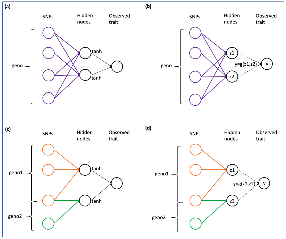
3. Flexibility
NN-MM can fit fully-connected neural networks ((a),(b)), or partial-connected neural networks ((c),(d)). Also, the relationship between middle layer (intermediate traits) and output layer (phenotypes) can be based on activation functions ((a),(c)), or pre-defined by a user-defined function ((b),(d)).
Network Types
| Type | Description | Use Case |
|---|---|---|
| (a) Fully-connected + Activation | All SNPs predict all omics; standard activation | General prediction |
| (b) Fully-connected + User-defined | All SNPs predict all omics; custom function | Domain-specific models |
| (c) Partial-connected + Activation | SNP groups predict specific omics; standard activation | Pathway analysis |
| (d) Partial-connected + User-defined | SNP groups predict specific omics; custom function | Advanced modeling |
4. Multi-threaded Parallelism
By default, multiple single-trait models will be used to model the relationships between input layer (genotypes) and middle layer (intermediate traits). Multi-threaded parallelism will be used for parallel computing. The number of threads can be checked by running Threads.nthreads() in Julia. Usually, using multiple threads will be about 3 times faster than using a single thread.
The number of execution threads is controlled by using the -t/--threads command-line argument (requires at least Julia 1.5).
For example, to start Julia with 4 threads:
julia --threads 4Or set the environment variable before starting Julia:
export JULIA_NUM_THREADS=4
julia
If you're using Juno via IDE like Atom, or VS Code with the Julia extension, multiple threads are typically loaded automatically based on system settings.
5. Quick Start
See the Tutorial for a complete walkthrough, or the Quick Start for a minimal example.
Minimal Example
using NNMM
using NNMM.Datasets
using DataFrames, CSV
using Random

Random.seed!(42)

# Load example data
geno_path = Datasets.dataset("genotypes_1000snps.txt", dataset_name="simulated_omics_data")
pheno_path = Datasets.dataset("phenotypes_sim.txt", dataset_name="simulated_omics_data")
pheno_df = CSV.read(pheno_path, DataFrame)

# Create data files
omics_df = pheno_df[:, vcat(:ID, [Symbol("omic$i") for i in 1:10])]
CSV.write("omics.csv", omics_df; missingstring="NA")
CSV.write("trait.csv", pheno_df[:, [:ID, :trait1]]; missingstring="NA")

# Define model
layers = [
    Layer(layer_name="geno", data_path=[geno_path]),
    Layer(layer_name="omics", data_path="omics.csv", missing_value="NA"),
    Layer(layer_name="pheno", data_path="trait.csv", missing_value="NA")
]

equations = [
    Equation(from_layer_name="geno", to_layer_name="omics",
             equation="omics = intercept + geno",
             traits=["omic$i" for i in 1:10], method="BayesC"),
    Equation(from_layer_name="omics", to_layer_name="pheno",
             equation="pheno = intercept + omics",
             traits=["trait1"], activation_function="linear")
]

# Run MCMC
results = runNNMM(layers, equations; chain_length=5000, burnin=1000)

# Cleanup
rm("omics.csv", force=true)
rm("trait.csv", force=true)
6. Tutorial Overview
| Part | Topic | Description |
|---|---|---|
| Part 2 | Basic NNMM | Fully-connected network with latent traits |
| Part 3 | NNMM with Omics | Incorporating observed omics data |
| Part 4 | Partial Networks | SNP groups → specific omics |
| Part 5 | Custom Functions | User-defined activation functions |
| Part 6 | Traditional GP | BayesC as NNMM special case |