Some Theory in JWAS
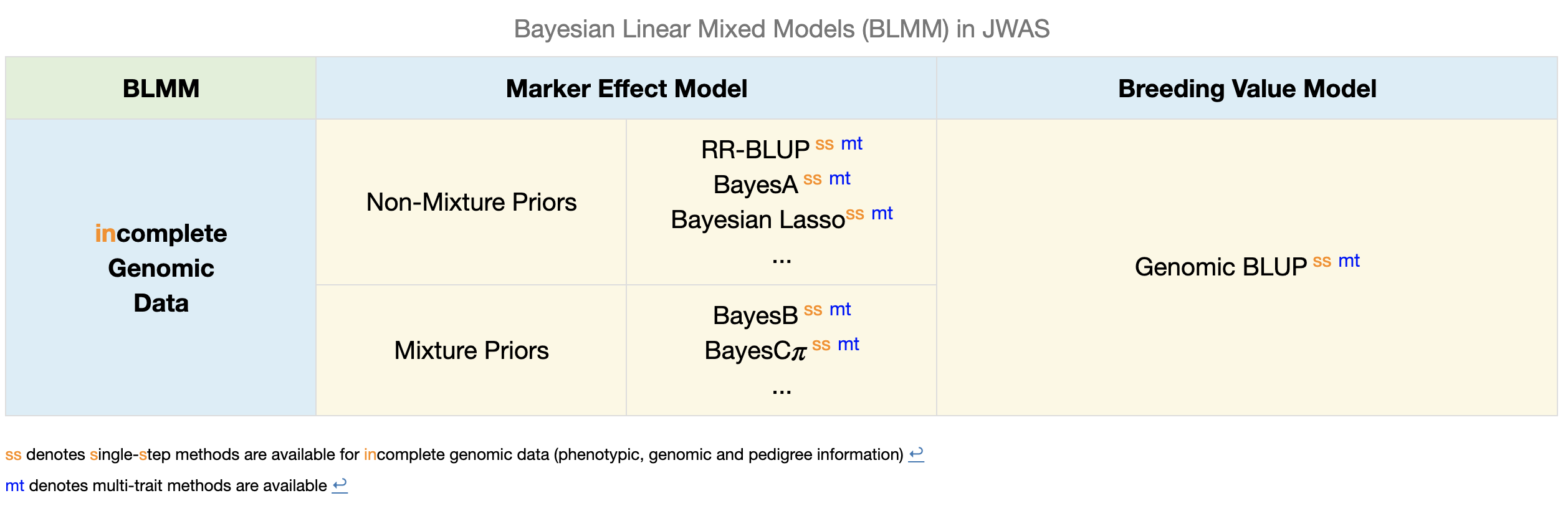
A Table for Bayesian Linear Mixed Models (BLMM)
Models
Complete Genomic Data
The general form of the multivariate (univariate) mixed effects model for individual $i$ from $n$ individuals with complete genomic data in JWAS is
\[ \mathbf{y}_{i} =\sum_{j=1}^{p_{b}}X_{ij}\mathbf{b}_{j}+\sum_{k=1}^{p_{u}}Z_{ik}\mathbf{u}_{k} +\sum_{l=1}^{p}M_{il}\boldsymbol{\alpha}_{l}+\mathbf{e}_{i}(1),\]
where $\mathbf{y}_{i}$ is a vector of phenotypes of $t$ traits for individual $i$; $X_{ij}$ is the incidence matrix covariate corresponding to the $j$th fixed effect for individual $i$; $\mathbf{b}_{j}$ is a vector of $j$th fixed effects for the $t$ traits; $Z_{ik}$ is the incidence matrix covariate corresponding to the $k$th random effect for individual $i$; $\boldsymbol{u}_{k}$ is a vector of the $k$th random effects of $t$ traits; $M_{il}$ is the genotype covariate at locus $l$ for individual $i$, $p$ is the number of genotyped loci (each coded as 0,1,2), $\boldsymbol{\alpha}_{l}$ is a vector of allele substitution effects or marker effects of $t$ traits for locus $j$, and $\mathbf{e}_{i}$ is the vector of random residual effects of $t$ traits for individual $i$. The JWAS implementation of this model involves missing phenotypes being imputed at each iteration of MCMC \cite{sorensenGianolaBook} so that all individuals have observations for all traits. Note that when the number of traits $t=1$, the general form above simplifies to the single-trait mixed effects model, and all vectors of effects in equation (1) become scalars.
Incomplete Genomic Data
The general form of the multivariate (univariate) mixed effects model with incomplete genomic data ("single-step" methods) for non-genotyped individuals is
\[\mathbf{y}_{i} =\sum_{j=1}^{p_{b}}X_{ij}\mathbf{b}_{j}+\sum_{k=1}^{p_{u}}Z_{ik}\mathbf{u}_{k}+ \sum_{l=1}^{p}\hat{M_{il}}\boldsymbol{\alpha}_{l}+\sum_{m=1}^{p_{\epsilon}}Z_{n[i,m]}\boldsymbol{\epsilon}_{m}+\boldsymbol{e}_{i} (2),\]
where $\mathbf{y}_{i}$ is a vector of phenotypes of $t$ traits for non-genotyped individual $i$; $\hat{{M}_{il}}$ is the imputed genotype covariate at locus $l$ for non-genotyped individual $i$, $Z_{n[i,m]}$ is the incidence matrix covariate corresponding to the $m$th imputation residual for individual $i$ and $\boldsymbol{\epsilon}_i$ is a vector of imputation residuals. $W_{im}$ is the incidence matrix covariate corresponding to the $m$th random effect for individual $i$. That vector of imputation residuals, $\boldsymbol{\epsilon}=\begin{bmatrix}\boldsymbol{\epsilon}_{1}^{T} & \boldsymbol{\epsilon}_{2}^{T} & \ldots & \end{bmatrix}^{T}$, are a priori assumed to be $N\left(0,(\mathbf{A}_{nn}-\mathbf{A}_{ng}\mathbf{A}_{gg}^{-1}\mathbf{A}_{gn})\otimes\mathbf{G}_{g}\right)$, where $\mathbf{A}_{nn}$ is the partition of the numerator relationship matrix $\mathbf{A}$ that corresponds to non-genotyped individuals, $\mathbf{A}_{ng}$ or its transpose $\mathbf{A}_{gn}$ are partitions of $\mathbf{A}$ corresponding to relationships between non-genotyped and genotyped individuals or vice versa, $\mathbf{A}_{gg}$ is the partition of $\mathbf{A}$ that corresponds to genotyped animals, and $\mathbf{G}_{g}$ is the additive genetic covariance matrix. All the other variables are the same as in equation (1).
Priors
Priors for effects other than markers
The fixed effects are assigned flat priors. The vector of random effects, $\mathbf{u}=\begin{bmatrix}\mathbf{u}_{1}^{T} & \mathbf{u}_{2}^{T} & \ldots & \mathbf{u}_{p_{2}}^{T}\end{bmatrix}^{T}$, are a priori assumed to be $N\left(0,\mathbf{A}\otimes\mathbf{G}\right)$ with various options for $\mathbf{A}$. For example, $\mathbf{A}$ could be an identity matrix if $\boldsymbol{u}_{k}$ is assumed to be independently and identically distributed. $\mathbf{A}$ can be the numerator relationship matrix, when $\boldsymbol{u}$ is a vector of polygenic effects and $\mathbf{G}$ represents the additive-genetic variance not explained by molecular markers. Note that $\boldsymbol{u}$ can also be a concatenation of vectors of different types of random effects, such as litter, pen, polygenic and maternal effects. The vector $\boldsymbol{e}_{i}$ of residuals are a priori assumed to be independently and identically following multivariate normal distributions with null mean and covariance matrix $\mathbf{R}$, which in turn is a priori assumed to have an inverse Wishart prior distribution, $W_{t}^{-1}\left(\mathbf{S}_{e},\nu_{e}\right)$. Note that when number of traits $t=1$, the priors for $\mathbf{G}$ and $\mathbf{R}$ in single-trait analyses follow scaled inverted chi-square distributions.
Priors for marker effects
single-trait BayesA
The prior assumption is that marker effects have identical and independent univariate-t distributions each with a null mean, scale parameter $S^2_{\alpha}$ and $\nu$ degrees of freedom. This is equivalent to assuming that the marker effect at locus $i$ has a univariate normal with null mean and unknown, locus-specific variance $\sigma^2_i$, which in turn is assigned a scaled inverse chi-square prior with scale parameter $S^2_{\alpha}$ and $\nu_{\alpha}$ degrees of freedom.
single-trait BayesB
In BayesB, the prior assumption is that marker effects have identical and independent mixture distributions, where each has a point mass at zero with probability $\pi$ and a univariate-t distribution with probability $1-\pi$ having a null mean, scale parameter $S^2_{\alpha}$ and $\nu$ degrees of freedom. Thus, BayesA is a special case of BayesB with $\pi=0$. Further, as in BayesA, the t-distribution in BayesB is equivalent to a univariate normal with null mean and unknown, locus-specific variance, which in turn is assigned a scaled inverse chi-square prior with scale parameter $S^2_{\alpha}$ and $\nu_{\alpha}$ degrees of freedom. (A fast and efficient Gibbs sampler was implemented for BayesB in JWAS.)
single-trait BayesC and BayesC$\pi$
In BayesC, the prior assumption is that marker effects have identical and independent mixture distributions, where each has a point mass at zero with probability $\pi$ and a univariate-normal distribution with probability $1-\pi$ having a null mean and variance $\sigma^2_{\alpha}$, which in turn has a scaled inverse chi-square prior with scale parameter $S^2_{\alpha}$ and $\nu_{\alpha}$ degrees of freedom. In addition to the above assumptions, in BayesC $\pi$, $\pi$ is treated as unknown with a uniform prior.
multiple-trait Bayesian Alphabet
In multi-trait BayesC$\Pi$, the prior for $\alpha_{lk}$, the marker effect of trait $k$ for locus $l$, is a mixture with a point mass at zero and a univariate normal distribution conditional on $\sigma_{k}^{2}$:
\[\alpha_{lk}\mid\pi_{k},\sigma_{k}^{2} \begin{cases} \sim N\left(0,\,\sigma_{k}^{2}\right) & \:probability\;(1-\pi_{k})\\ 0 & \:probability\;\pi_{k} \end{cases}\]
and the covariance between effects for traits $k$ and $k'$ at the same locus, i.e., $\alpha_{lk}$ and $\alpha_{lk^{'}}$ is
\[cov\left(\alpha_{lk},\alpha_{lk^{'}}\mid\sigma_{kk^{'}}\right)=\begin{cases} \sigma_{kk^{'}} & \:if\:both\,\alpha_{lk}\neq0\:and\:\alpha_{lk^{'}}\neq0\\ 0 & \:otherwise \end{cases}.\]
The vector of marker effects at a particular locus $\boldsymbol{\alpha}_{l}$ is written as $\boldsymbol{\alpha}_{l}=\boldsymbol{D}_{l}\boldsymbol{\beta}_{l}$, where $\boldsymbol{D}_{l}$ is a diagonal matrix with elements $diag\left(\boldsymbol{D}_{l}\right)=\boldsymbol{\delta}_{l}=\left(\delta_{l1},\delta_{l2},\delta_{l3}\ldots\delta_{lt}\right)$, where $\delta_{lk}$ is an indicator variable indicating whether the marker effect of locus $l$ for trait $k$ is zero or non-zero, and the vector $\boldsymbol{\beta}_{l}$ follows a multivariate normal distribution with null mean and covariance matrix $\boldsymbol{G}$. The covariance matrix $\boldsymbol{G}$ is $a$ $priori$ assumed to follow an inverse Wishart distribution, $W_{t}^{-1}\left(\mathbf{S}_{\beta},\nu_{\beta}\right)$.
In the most general case, any marker effect might be zero for any possible combination of $t$ traits resulting in $2^{t}$ possible combinations of $\boldsymbol{\delta}_{l}$. For example, in a $t$=2 trait model, there are $2^{t}=4$ combinations for $\boldsymbol{\delta}_{l}$: $(0,\,0)$, $(0,\,1)$, $(1,\,0)$, $(1,\,1)$. Suppose in general we use numerical labels "1", "2",$\ldots$, "$l$" for the $2^{t}$ possible outcomes for $\boldsymbol{\delta}_{l}$, then the prior for $\boldsymbol{\delta}_{l}$ is a categorical distribution
\[p\left(\boldsymbol{\delta}_{l}=``i"\right)= \Pi_{1}I\left(\boldsymbol{\delta}_{l}=``1"\right)+\Pi_{2}I\left(\boldsymbol{\delta}_{l}=``2"\right)+...+\Pi_{l}I\left(\boldsymbol{\delta}_{l}=``l"\right),\]
where $\sum_{i=1}^{l}\Pi_{i}=1$ with $\Pi_{i}$ being the prior probability that the vector $\boldsymbol{\delta}_{l}$ corresponds to the vector labelled $"i"$. A Dirichlet distribution with all parameters equal to one, i.e., a uniform distribution, can be used for the prior for $\boldsymbol{\Pi}=\left(\Pi_{1},\Pi_{2},...,\Pi_{l}\right)$.
The differences in multi-trait BayesB method is that the prior for $\boldsymbol{\beta}_{l}$ is a multivariate t distribution, rather than a multivariate normal distribution. This is equivalent to assuming $\boldsymbol{\beta}_{l}$ has a multivariate normal distribution with null mean and locus-specific covariance matrix $\boldsymbol{G}_{l}$, which is assigned an inverse Wishart prior, $W_{t}^{-1}\left(\mathbf{S}_{\beta},\nu_{\beta}\right)$. Multi-trait BayesA method is a special case of multi-trait BayesB method where $\boldsymbol{\delta}_{l}$ is always a vector of ones.
references
- Meuwissen T, Hayes B, Goddard M. Prediction of total genetic value using genome-wide dense marker maps. Genetics, 2001,157:1819–1829.
- Fernando R, Garrick D. Bayesian methods applied to GWAS. Methods Mol Biol. 2013, 1019:237–274.
- Cheng H, Garrick D, Fernando R. A fast and efficient Gibbs sampler for BayesB in whole- genome analyses. Genetics Selection Evolution, 2015, 47:80.
- Fernando R, Dekkers J, Garrick D. A class of Bayesian methods to combine large numbers of genotyped and non-genotyped animals for whole-genome analyses. Genetics Selection Evolution, 2015, 46(1), 50.
- Fernando R, Cheng H, Golden B, Garrick D.. Computational strategies for alternative single-step Bayesian regression models with large numbers of genotyped and non-genotyped animals. Genetics Selection Evolution, 2016, 48(1), 96.
- Cheng H, Kizilkaya K, Zeng J, Garrick D, Fernando R. Genomic Prediction from Multiple-trait Bayesian Regression Methods using Mixture Priors. Genetics. 2018, 209(1).