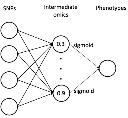
Mixed effect neural network: Genotypes -> (complete/incomplete) Intemediate omics features -> Phenotyes
Tips:
- Put the names of omics features in the
build_model()function through thelatent_traitsargument. - If there are many omics features (e.g., 1000), it is recommanded to set
printout_model_info=falsein therunMCMC()function. - Missing omics data for individuals in the training dataset (i.e., individuals with phenotypes) is allowed. When you read a file with missing values via the
CSV.read()function, themissingstringsargument should be used to set sentinel values that will be parsed asmissing. - For individuals in the testing dataset (i.e., individuals without phenotypes), if the testing individuals have complete omics data, then incorporating the omics data of those individuals may improve the relationship between input layer (genotype) and middle layer (omics).
example(o1): fully-connected neural networks with observed intemediate omics features
- nonlinear function (to define relationship between omics and phenotye): sigmoid (other supported activation functions: "tanh", "relu", "leakyrelu", "linear")
- number of omics features in the middle layer: 10
- Bayesian model: multiple independent single-trait BayesC (to sample marker effects on intemediate omics)
- sample the missing omics in the middle layer: Hamiltonian Monte Carlo

# Step 1: Load packages
using JWAS,DataFrames,CSV,Statistics,JWAS.Datasets, Random, HTTP #HTTP to download demo data from github
Random.seed!(123)

# Step 2: Read data (from github)
phenofile  = HTTP.get("https://raw.githubusercontent.com/zhaotianjing/nnmm_doc/main/data_simulation/y.csv").body
omicsfile  = HTTP.get("https://raw.githubusercontent.com/zhaotianjing/nnmm_doc/main/data_simulation/omics.csv").body
genofile   = HTTP.get("https://raw.githubusercontent.com/zhaotianjing/nnmm_doc/main/data_simulation/geno_n100_p200.csv").body
phenotypes = CSV.read(phenofile,DataFrame)
omics      = CSV.read(omicsfile,DataFrame)
geno_df    = CSV.read(genofile,DataFrame)

omics_names = names(omics)[2:end]  #get names of omics
insertcols!(omics,2,:y => phenotypes[:,:y], :bv => phenotypes[:,:bv]) #phenotype and omics should be in the same dataframe

genotypes = get_genotypes(geno_df,separator=',',method="BayesC")

# Step 3: Build Model Equations
model_equation  ="y = intercept + genotypes" #name of phenotypes is "y"
                                             #name of genotypes is "genotypes" (user-defined in the previous step)
                                             #the single-trait mixed model used between input and each omics is: omics = intercept + genotypes
model = build_model(model_equation,
		    num_hidden_nodes=10,          #number of omics in middle layer is 3
                    latent_traits=omics_names,    #name of all omics
		    nonlinear_function="sigmoid") #sigmoid function is used to approximate relationship between omics and phenotypes

# Step 4: Run Analysis
out=runMCMC(model, omics, chain_length=5000, printout_model_info=false);

# Step 5: Check Accuruacy
results    = innerjoin(out["EBV_NonLinear"], omics, on = :ID)
accuruacy  = cor(results[!,:EBV],results[!,:bv])
Includes a residual that is not mediated by other omics features
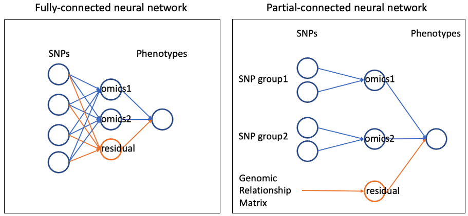
To include residuals polygenic component (i.e. directly from genotypes to phenotypes, not mediated by omics features), you can additional hidden nodes in the middle layer (see example (o2)). This can also be achieved in a partial-connected neural network in a same manner.

example(o2): fully-connected neural network with residuals
For all individuals, this extra hidden node will be treated as unknown to be sampled.
# Step 1: Load packages
using JWAS,DataFrames,CSV,Statistics,JWAS.Datasets, Random, HTTP
Random.seed!(123)

# Step 2: Read data (from github)
phenofile  = HTTP.get("https://raw.githubusercontent.com/zhaotianjing/nnmm_doc/main/data_simulation/y.csv").body
omicsfile  = HTTP.get("https://raw.githubusercontent.com/zhaotianjing/nnmm_doc/main/data_simulation/omics.csv").body
genofile   = HTTP.get("https://raw.githubusercontent.com/zhaotianjing/nnmm_doc/main/data_simulation/geno_n100_p200.csv").body
phenotypes = CSV.read(phenofile,DataFrame)
omics      = CSV.read(omicsfile,DataFrame)
geno_df    = CSV.read(genofile,DataFrame)

insertcols!(omics, :residual => missing)  #create a hidden node to account for residuals
omics[!,:residual] = convert(Vector{Union{Missing,Float64}}, omics[!,:residual]) #transform the datatype is required for Julia
omics_names = names(omics)[2:end]  #get names of 10 omics and 1 hidden node
insertcols!(omics,2,:y => phenotypes[:,:y], :bv => phenotypes[:,:bv]) #phenotype and omics should be in the same dataframe

genotypes = get_genotypes(geno_df,separator=',',method="BayesC")

# Step 3: Build Model Equations
model_equation  ="y = intercept + genotypes"
model = build_model(model_equation,
		    num_hidden_nodes=11,   #10 omcis and 1 hidden node
                    latent_traits=omics_names,
		    nonlinear_function="sigmoid")

# Step 4: Run Analysis
out = runMCMC(model,omics,chain_length=5000,printout_model_info=false)

# Step 5: Check Accuruacy
results    = innerjoin(out["EBV_NonLinear"], omics, on = :ID)
accuruacy  = cor(results[!,:EBV],results[!,:bv])
Users can also add extra hidden nodes in the partial-connected neural network. Please check next documentation for building a partial-connected neural network.
Output files
Same as those described in Part2.
Julia Tips:
- You may want to set missing values manually, for example, setting the phenotypes for individuals in testing dataset as
missing. Firstly, the type of columns should be changed to allowmissing, e.g.,phenotypes[!,:y] = convert(Vector{Union{Missing,Float64}}, phenotypes[!,:y]). Then,missingcan be set manually, e.g.,phenotypes[10:11,:y1] .= missingforces the 10th and 11th elements to bemissing.